# Introducing Q-Learning [[q-learning]]
## What is Q-Learning? [[what-is-q-learning]]
Q-Learning is an **off-policy value-based method that uses a TD approach to train its action-value function:**
- *Off-policy*: we'll talk about that at the end of this chapter.
- *Value-based method*: finds the optimal policy indirectly by training a value or action-value function that will tell us **the value of each state or each state-action pair.**
- *Uses a TD approach:* **updates its action-value function at each step instead of at the end of the episode.**
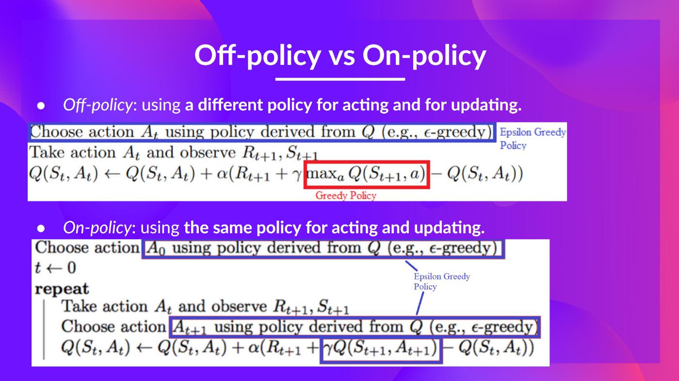
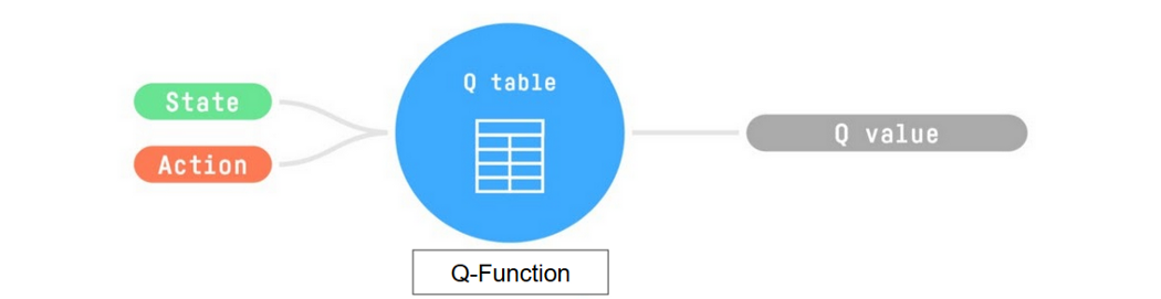
**Q-Learning is the algorithm we use to train our Q-Function**, an **action-value function** that determines the value of being at a particular state and taking a specific action at that state.
Given a state and action, our Q Function outputs a state-action value (also called Q-value)
The **Q comes from "the Quality" of that action at that state.**
Internally, our Q-function has **a Q-table, a table where each cell corresponds to a state-action value pair value.** Think of this Q-table as **the memory or cheat sheet of our Q-function.**
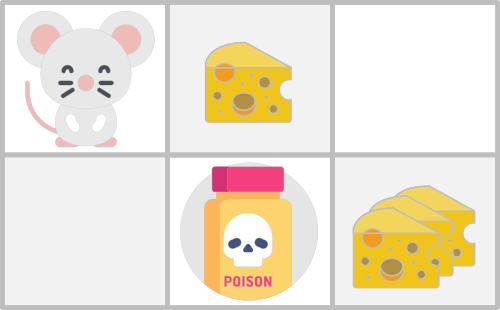
If we take this maze example:
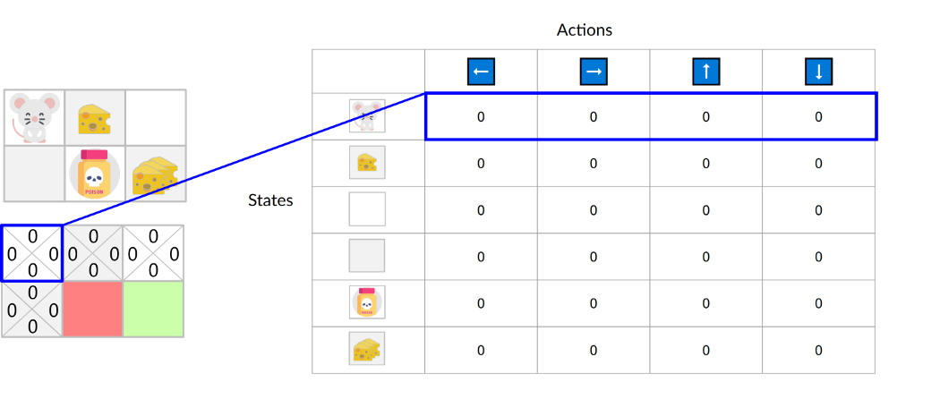
The Q-Table is initialized. That's why all values are = 0. This table **contains, for each state, the four state-action values.**
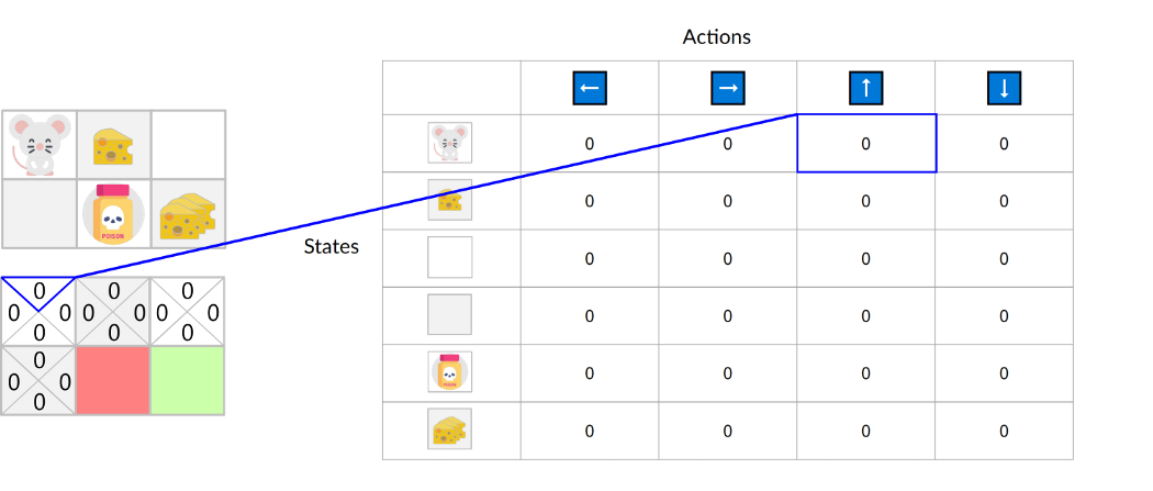
Here we see that the **state-action value of the initial state and going up is 0:**
Therefore, Q-function contains a Q-table **that has the value of each-state action pair.** And given a state and action, **our Q-Function will search inside its Q-table to output the value.**
Given a state and action pair, our Q-function will search inside its Q-table to output the state-action pair value (the Q value).
If we recap, *Q-Learning* **is the RL algorithm that:**
- Trains *Q-Function* (an **action-value function**) which internally is a *Q-table* **that contains all the state-action pair values.**
- Given a state and action, our Q-Function **will search into its Q-table the corresponding value.**
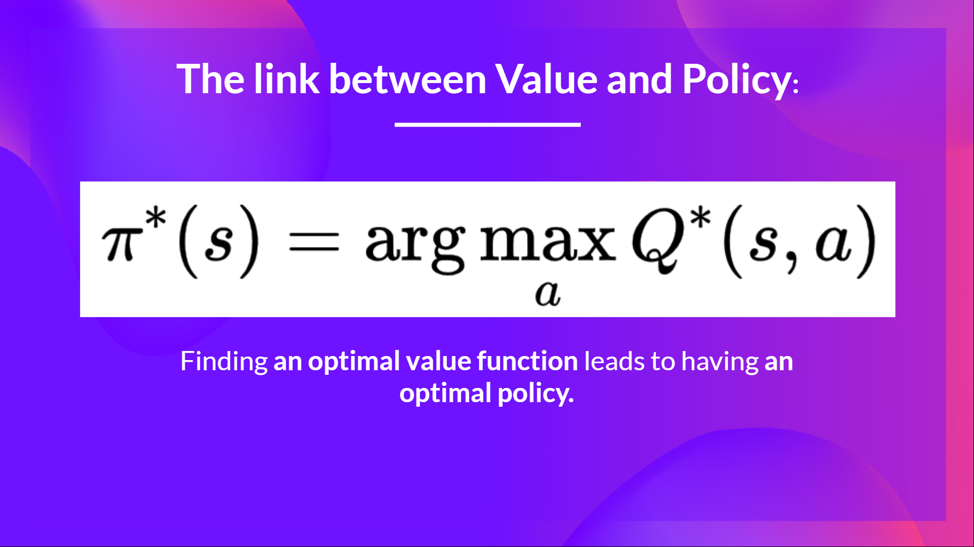
- When the training is done, **we have an optimal Q-function, which means we have optimal Q-Table.**
- And if we **have an optimal Q-function**, we **have an optimal policy** since we **know for each state what is the best action to take.**
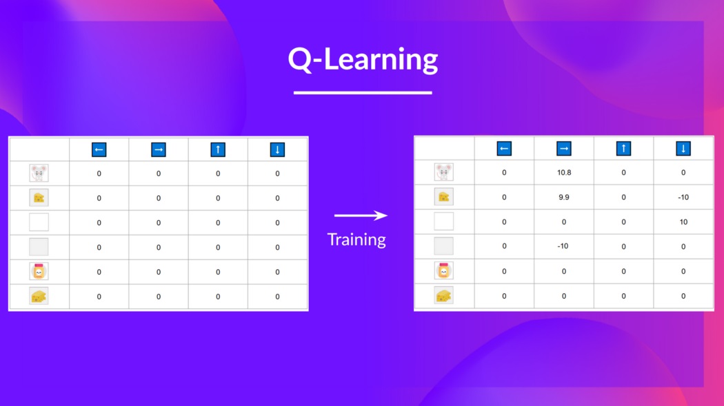
But, in the beginning, **our Q-Table is useless since it gives arbitrary values for each state-action pair** (most of the time, we initialize the Q-Table to 0 values). But, as we'll **explore the environment and update our Q-Table, it will give us better and better approximations.**
We see here that with the training, our Q-Table is better since, thanks to it, we can know the value of each state-action pair.
So now that we understand what Q-Learning, Q-Function, and Q-Table are, **let's dive deeper into the Q-Learning algorithm**.
## The Q-Learning algorithm [[q-learning-algo]]
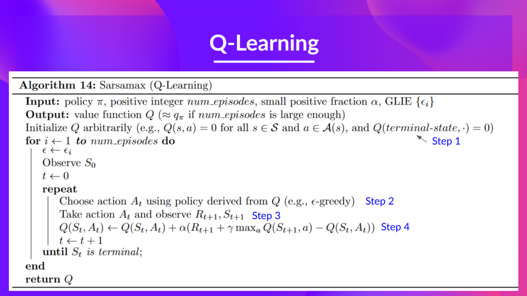
This is the Q-Learning pseudocode; let's study each part and **see how it works with a simple example before implementing it.** Don't be intimidated by it, it's simpler than it looks! We'll go over each step.
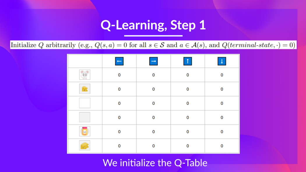
### Step 1: We initialize the Q-Table [[step1]]
We need to initialize the Q-Table for each state-action pair. **Most of the time, we initialize with values of 0.**
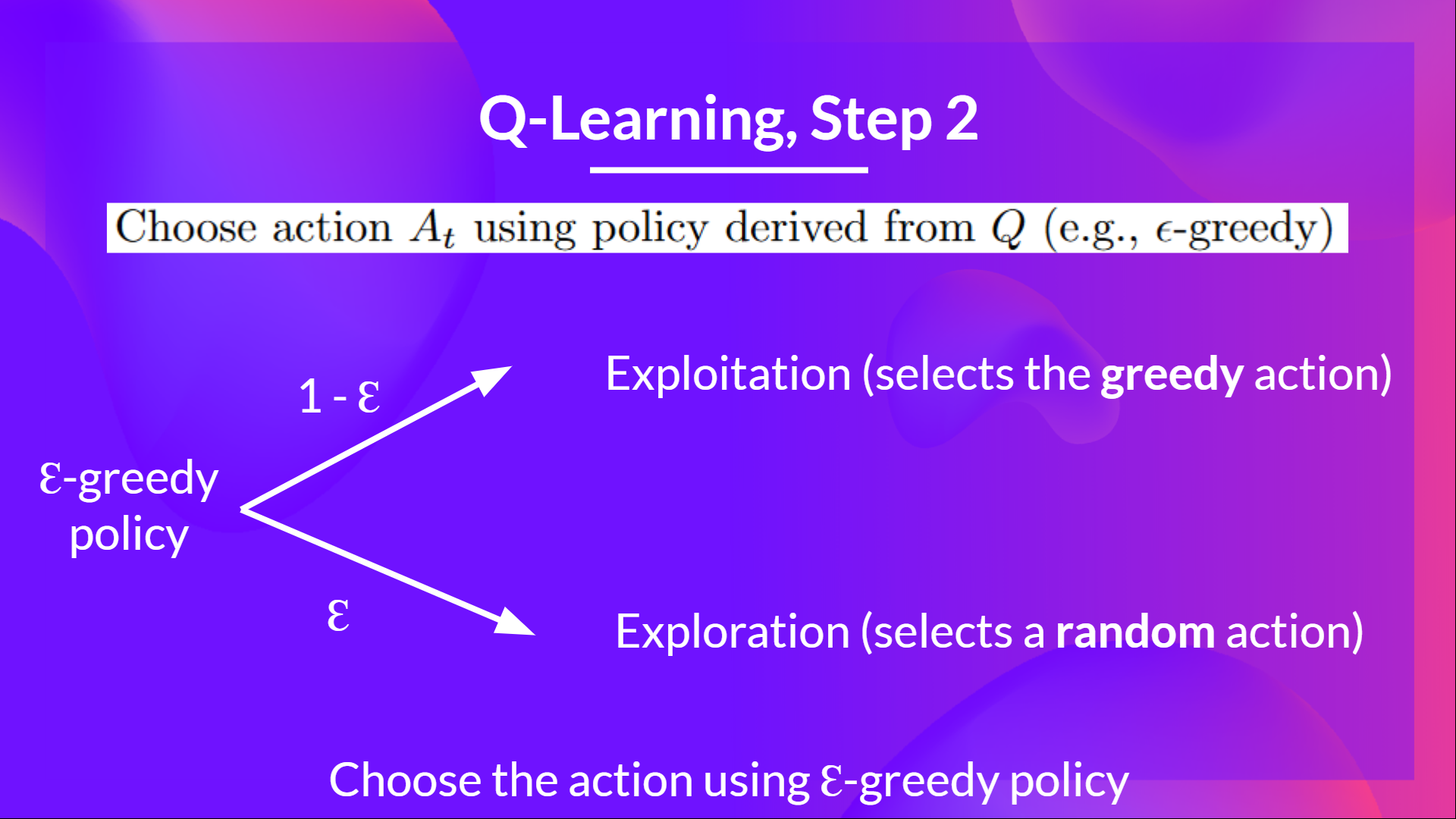
### Step 2: Choose action using Epsilon Greedy Strategy [[step2]]
Epsilon Greedy Strategy is a policy that handles the exploration/exploitation trade-off.
The idea is that we define epsilon ɛ = 1.0:
- *With probability 1 — ɛ* : we do **exploitation** (aka our agent selects the action with the highest state-action pair value).
- With probability ɛ: **we do exploration** (trying random action).
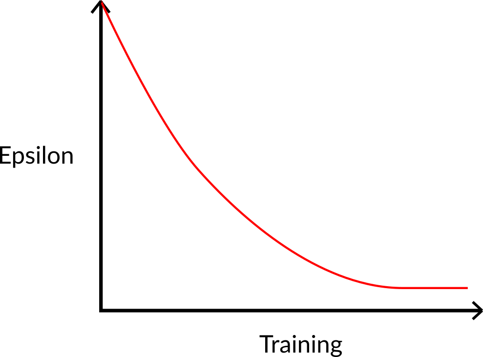
At the beginning of the training, **the probability of doing exploration will be huge since ɛ is very high, so most of the time, we'll explore.** But as the training goes on, and consequently our **Q-Table gets better and better in its estimations, we progressively reduce the epsilon value** since we will need less and less exploration and more exploitation.
### Step 3: Perform action At, gets reward Rt+1 and next state St+1 [[step3]]
### Step 4: Update Q(St, At) [[step4]]
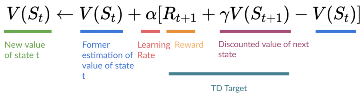
Remember that in TD Learning, we update our policy or value function (depending on the RL method we choose) **after one step of the interaction.**
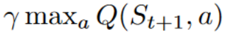
To produce our TD target, **we used the immediate reward \\(R_{t+1}\\) plus the discounted value of the next state best state-action pair** (we call that bootstrap).
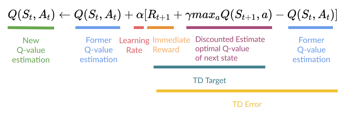
Therefore, our \\(Q(S_t, A_t)\\) **update formula goes like this:**
It means that to update our \\(Q(S_t, A_t)\\):
- We need \\(S_t, A_t, R_{t+1}, S_{t+1}\\).
- To update our Q-value at a given state-action pair, we use the TD target.
How do we form the TD target?
1. We obtain the reward after taking the action \\(R_{t+1}\\).
2. To get the **best next-state-action pair value**, we use a greedy policy to select the next best action. Note that this is not an epsilon greedy policy, this will always take the action with the highest state-action value.
Then when the update of this Q-value is done. We start in a new_state and select our action **using our epsilon-greedy policy again.**
**It's why we say that this is an off-policy algorithm.**
## Off-policy vs On-policy [[off-vs-on]]
The difference is subtle:
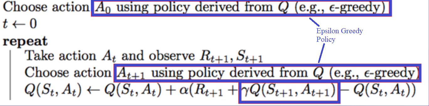
- *Off-policy*: using **a different policy for acting and updating.**
For instance, with Q-Learning, the Epsilon greedy policy (acting policy), is different from the greedy policy that is **used to select the best next-state action value to update our Q-value (updating policy).**
Acting Policy
Is different from the policy we use during the training part:
Updating policy
- *On-policy:* using the **same policy for acting and updating.**
For instance, with Sarsa, another value-based algorithm, **the Epsilon-Greedy Policy selects the next_state-action pair, not a greedy policy.**
Sarsa
 The Q-Table is initialized. That's why all values are = 0. This table **contains, for each state, the four state-action values.**
 Here we see that the **state-action value of the initial state and going up is 0:**
 Therefore, Q-function contains a Q-table **that has the value of each-state action pair.** And given a state and action, **our Q-Function will search inside its Q-table to output the value.**
 But, in the beginning, **our Q-Table is useless since it gives arbitrary values for each state-action pair** (most of the time, we initialize the Q-Table to 0 values). But, as we'll **explore the environment and update our Q-Table, it will give us better and better approximations.**
 ### Step 1: We initialize the Q-Table [[step1]]
 We need to initialize the Q-Table for each state-action pair. **Most of the time, we initialize with values of 0.**
### Step 2: Choose action using Epsilon Greedy Strategy [[step2]]
We need to initialize the Q-Table for each state-action pair. **Most of the time, we initialize with values of 0.**
### Step 2: Choose action using Epsilon Greedy Strategy [[step2]]
 Epsilon Greedy Strategy is a policy that handles the exploration/exploitation trade-off.
The idea is that we define epsilon ɛ = 1.0:
- *With probability 1 — ɛ* : we do **exploitation** (aka our agent selects the action with the highest state-action pair value).
- With probability ɛ: **we do exploration** (trying random action).
At the beginning of the training, **the probability of doing exploration will be huge since ɛ is very high, so most of the time, we'll explore.** But as the training goes on, and consequently our **Q-Table gets better and better in its estimations, we progressively reduce the epsilon value** since we will need less and less exploration and more exploitation.
Epsilon Greedy Strategy is a policy that handles the exploration/exploitation trade-off.
The idea is that we define epsilon ɛ = 1.0:
- *With probability 1 — ɛ* : we do **exploitation** (aka our agent selects the action with the highest state-action pair value).
- With probability ɛ: **we do exploration** (trying random action).
At the beginning of the training, **the probability of doing exploration will be huge since ɛ is very high, so most of the time, we'll explore.** But as the training goes on, and consequently our **Q-Table gets better and better in its estimations, we progressively reduce the epsilon value** since we will need less and less exploration and more exploitation.
 ### Step 3: Perform action At, gets reward Rt+1 and next state St+1 [[step3]]
 ### Step 4: Update Q(St, At) [[step4]]
Remember that in TD Learning, we update our policy or value function (depending on the RL method we choose) **after one step of the interaction.**
To produce our TD target, **we used the immediate reward \\(R_{t+1}\\) plus the discounted value of the next state best state-action pair** (we call that bootstrap).
### Step 4: Update Q(St, At) [[step4]]
Remember that in TD Learning, we update our policy or value function (depending on the RL method we choose) **after one step of the interaction.**
To produce our TD target, **we used the immediate reward \\(R_{t+1}\\) plus the discounted value of the next state best state-action pair** (we call that bootstrap).
 Therefore, our \\(Q(S_t, A_t)\\) **update formula goes like this:**
 It means that to update our \\(Q(S_t, A_t)\\):
- We need \\(S_t, A_t, R_{t+1}, S_{t+1}\\).
- To update our Q-value at a given state-action pair, we use the TD target.
How do we form the TD target?
1. We obtain the reward after taking the action \\(R_{t+1}\\).
2. To get the **best next-state-action pair value**, we use a greedy policy to select the next best action. Note that this is not an epsilon greedy policy, this will always take the action with the highest state-action value.
Then when the update of this Q-value is done. We start in a new_state and select our action **using our epsilon-greedy policy again.**
**It's why we say that this is an off-policy algorithm.**
## Off-policy vs On-policy [[off-vs-on]]
The difference is subtle:
- *Off-policy*: using **a different policy for acting and updating.**
For instance, with Q-Learning, the Epsilon greedy policy (acting policy), is different from the greedy policy that is **used to select the best next-state action value to update our Q-value (updating policy).**
It means that to update our \\(Q(S_t, A_t)\\):
- We need \\(S_t, A_t, R_{t+1}, S_{t+1}\\).
- To update our Q-value at a given state-action pair, we use the TD target.
How do we form the TD target?
1. We obtain the reward after taking the action \\(R_{t+1}\\).
2. To get the **best next-state-action pair value**, we use a greedy policy to select the next best action. Note that this is not an epsilon greedy policy, this will always take the action with the highest state-action value.
Then when the update of this Q-value is done. We start in a new_state and select our action **using our epsilon-greedy policy again.**
**It's why we say that this is an off-policy algorithm.**
## Off-policy vs On-policy [[off-vs-on]]
The difference is subtle:
- *Off-policy*: using **a different policy for acting and updating.**
For instance, with Q-Learning, the Epsilon greedy policy (acting policy), is different from the greedy policy that is **used to select the best next-state action value to update our Q-value (updating policy).**